 Offsite links

-The Reyes Rendering Architecture-
Part two.
In part one, we covered the first three steps of the Reyes rendering architecture: bounding, splitting, and dicing. This article will cover the remaining two steps: shading and samping.
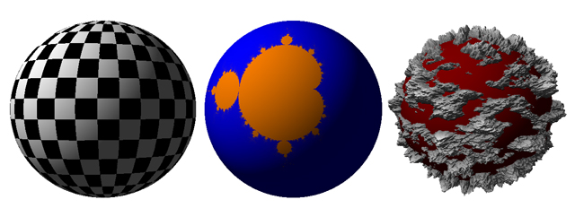
Shading
Recall that every primitive is diced into a grid of micropolygons with a density of approximately one micropolygon per pixel. The small size of the micropolygons drastically simplifies many aspects of shading. For example, there's no need to interpolate texture coordinates or normals.
The actual shading loop very simple. A basic dot product light model might be implemented like this:
void Shade(MicroGrid *grid)
{
   for(int u=0; u < grid->Width()-1; u++)
   {
      for(int v=0; v < grid->Height()-1; v++)
      {
         p3d n = grid->GetNormal(u, v);
         Colour c = Colour(0.5,1,0.5) *
                        max(0.2, n.dot( p3d(1, 1, -1).normalize()));
         grid->SetColour(u, v, c);
      }
   }
}
This functions simply attenuates each micropolygon's colour based upon the dot product of its normal and the light direction. It should be familiar to almost everyone whose had any experience with 3d rendering algorithms in the past.
Reyes provides and extremely flexible framework for defining surface appearance; There is practically no limit to what you can do inside a surface shader. This flexibility is one of the reasons that Pixar's Reyes based Photorealistic Renderman became so dominant in the CG special effects business. Allowing artists to define the appearance of surfaces without being constrained to simple mathematical models of light was a major step forward in the 1980's when Renderman was released.
The code given above isn't the most effiecient way to shade surfaces in Reyes. Not by a long shot. Shading in Reyes can be made parallel quite easily. Because it has no branches, the above code could be directly translated into vector code simply by replacing each operation with its eight-wide SSE equivalent for example.
Shading in Reyes based renderers is usually done with a purpose built language like the RenderMan Shading Language. This allows new shaders to be written without needing to recompile the renderer. It also allows shaders written in one renderer to be used in any other renderer that supports the same shading language. Because of the SIMD friendly nature of shading in Reyes, using an interpreted shading language can be nearly as fast and compiled shaders. The overhead of the shader virtual machine can be amortized over thousands of micropolygons allowing a drastic reduction in the amount of computing power needed.
Shader compilers and shading languages are a bit beyond the scope of this article though. They'll just have wait until some future installment.
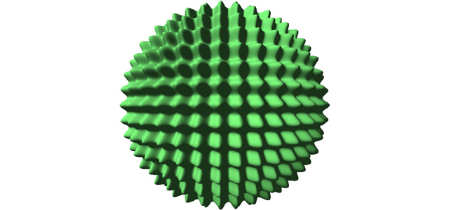
Displacement
Setting each micropolygon's colour isn't such a large departure from other rendering algorithms. The ability to modify the location of the vertices in the microgrid is perhaps more interesting from our perspective. This is called displacement mapping, and is one of Reyes' biggest strengths when compared to other rendering algorithms.
A simple displacement shader that modifies each vertice's location based upon its x and y coordinates might look like this:
void Displace(Microgrid *grid)
{
   for(int u=0; uW(); u++)
   {
      for(int v=0; vH(); v++)
      {
         p3d vert = grid->GetVertex(u,v);
         p3d n = grid->GetNormal(u,v);

         vert+=n*sin(vert.x*30)*0.045f,
         vert+=n*cos(vert.y*30)*0.045f

         grid->SetVertex(u,v, vert);
      }
   }

   grid->RecomputNormals();
}
It's important to recompute the microgrid's normals before shading.
Displacement can cause a number of problems if not accounted for in the bound/split pipeline. Surfaces that are normally outside the screen bounding volume might not be when displaced. Large displacements can also cause sub-pixel sized micropolygons on the undisplaced surface to become larger than one pixel. An extreme example would be a sphere that is normally a few pixels across, but becomes several hundred pixels wide under displacement. Accounting for both these issues only involves adding a call the the displacements shader in the bounding function.
void Bound(Primitive *shape, BoundingBox *bbox, Microgrid *grid)
{
   //Coarsely dice the primitive
   dice(shape, grid, 8, 8);

   //Account for displacement
   if(shape->displaced)
      Displace(grid);

   //Project the vertices of the micropolygons onto the screen
   project_microgrid(grid);

  ...
}
There is one major issue when displacing geometry: Step functions in the displacement shader. Step functions result in large micropolygons. Because step functions are infinitely "thin", they can never be split. This means that any shapes with them may never leave the bound/split phase.

There are various ways you could combat this. The simplest way is to prevent a shape being split more than a set number of times.
bool Splittable(Primitive *current_object,
                SplitDirection &direction)
{
   //If current_object is too "old", mark it as unsplittable
   if(current_object->generation > max_generations)
   {
      return false;
   }

   Microgrid grid;
   dice(current_object, &grid, 8, 8);

   ...
}
The splitting function will need to be modified slightly to keep track of each object's age:
void Split(Primitive *current_object,
             Primitive *child_1,
             Primitive *child_2,
             SplitDirection split_direction)
{
   child_1->control_points = current_object->control_points;
   child_2->control_points = current_object->control_points;

   //Add age to new primitives...
   child_1->generation = child_2->generation =
   current_object->generation+1;

   if(split_direction == VSplit)
   {
   ...
Busting and Sampling
After a grid has been displaced and shaded, its vertice are projected onto the screen using the same projection function as the bound/split pipeline. After the grid has been projected, it is "busted" into individual quadrilaterals which are then sampled in screen space.
Sampling each micropolygon involves looping over its screen space bounding box and running a simple 2D inside-outside polygon test.